Importance reweighting example

   """
   Script to test importance reweighting


   In this script we generate data according to

     y = m x + c + Normal(0, sigma)

   Then

   1) Calculate the "full" posterior P(m, c | data)
   2) Calculate the "partial" posterior P(m | data, c=0) (note c=0 in the injection)
   3) Use importance reweighting to calculate P(m| data) from the "partial" results

   """
   import matplotlib.pyplot as plt
   import numpy as np
   import bilby
   from scipy.special import logsumexp
   import tqdm

   np.random.seed(1234)
   outdir = '.'
   sampler = 'dynesty'
   npoints = 5000


   def marginalized_log_likelihood_over_c(m, likelihood):
       """ Calculates L(data| m), marginalized over c

       Parameters
       ----------
       m: float
           The fixed value of m at which to calculate the marginalized likelihood
       likelihood: bilby.core.likelihood.Likelihood instance
           Used to evaluate the log likelihood

       Note
       ----
           Integration range chosen to cover the region of interest. Note, this
           neglects the normalization factors which don't count in the weight
           calculation.
       """
       likelihood.parameters['m'] = m
       c_array = np.linspace(-0.2, 0.2, 100)
       integrand = []
       for c in c_array:
           likelihood.parameters['c'] = c
           integrand.append(likelihood.log_likelihood())
       return logsumexp(integrand)


   def model(x, m, c):
       return m * x + c


   # Injection parameters and create data
   m = 1
   c = 0
   sigma = 0.1
   N = 100
   x = np.linspace(0, 1, N)
   y = model(x, m, c) + np.random.normal(0, sigma, N)

   likelihood = bilby.core.likelihood.GaussianLikelihood(x, y, model)

   # Run the full PE
   priors = dict()
   priors['m'] = bilby.core.prior.Uniform(0, 5, 'm')
   priors['c'] = bilby.core.prior.Uniform(-2, 2, 'c')
   priors['sigma'] = sigma
   full_result = bilby.run_sampler(
       likelihood=likelihood, priors=priors, sampler=sampler, npoints=npoints,
       outdir=outdir, label='full')
   full_result.plot_corner()

   # Run the constrained PE
   priors = dict()
   priors['m'] = bilby.core.prior.Uniform(0, 5, 'm')
   priors['c'] = 0
   priors['sigma'] = sigma
   partial_result = bilby.run_sampler(
       likelihood=likelihood, priors=priors, sampler=sampler, npoints=npoints,
       outdir=outdir, label='partial')
   partial_result.plot_corner()

   # Pull out the uniformly-weighted samples from the full and partial runs
   full_m_samples = full_result.posterior.m.values
   partial_m_samples = partial_result.posterior.m.values

   # Calculate primed likelihood
   log_likelihood_prime = []
   for m in tqdm.tqdm(partial_m_samples):
       log_likelihood_prime.append(marginalized_log_likelihood_over_c(m, likelihood))
   log_likelihood_prime = np.array(log_likelihood_prime)

   # Calculate p, the normalized probably for each sample in partial_m_samples
   log_likelihood = partial_result.posterior.log_likelihood.values
   weights = log_likelihood_prime - log_likelihood
   p = np.exp(weights)
   p /= np.sum(p)

   # Reweight to get corrected samples
   reweight_samples = np.random.choice(partial_m_samples, size=30000, p=p)

   # Plot
   bins = np.linspace(0.9, 1.1, 50)
   fig, ax = plt.subplots()
   ax.hist(full_m_samples, bins=bins, density=True, label="full",
           histtype='step', linewidth=2.5)
   ax.hist(partial_m_samples, bins=bins, density=True, alpha=0.5, label="partial")
   ax.hist(reweight_samples, bins=bins, density=True, alpha=0.5, label="resampled")
   ax.legend()
   ax.set_xlabel("m")
   plt.savefig("posterior")

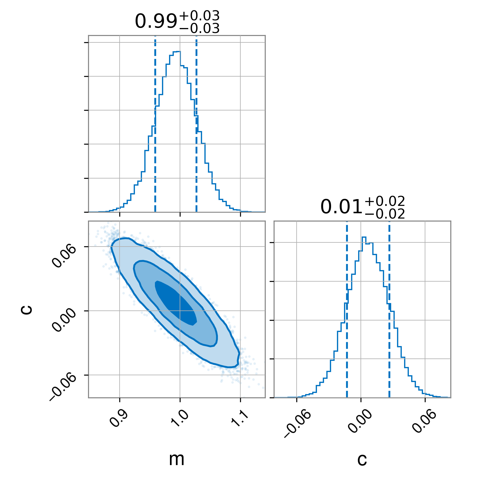
Having run this script, we obtain three images. First, the full posterior

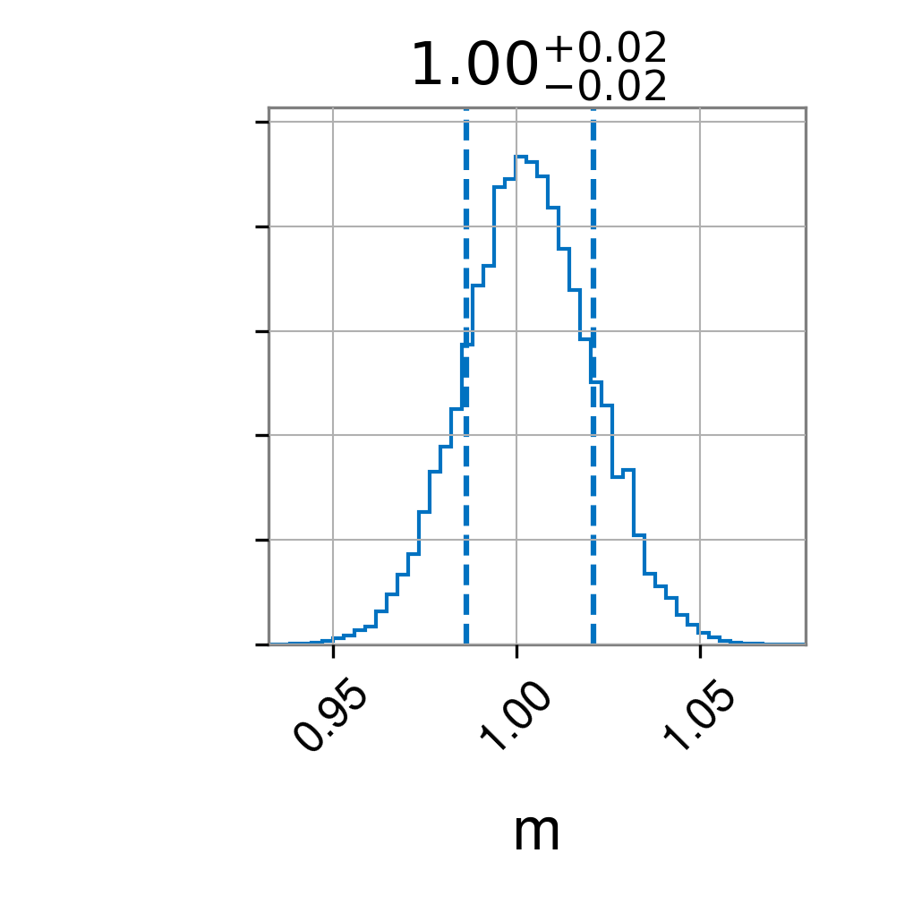
Second, the posterior when fixing c=0

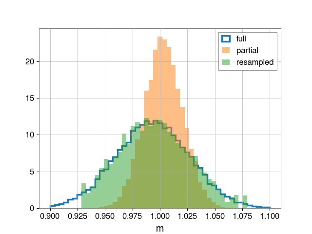
Finally, the rewighted posterior from fixed case